An Interactive Introduction to Reinforcement Learning

Reinforcement learning (RL) is a branch of machine learning that aim at finding an (hopefully) optimal policy (or behavior) for an agent in a given environment. I find it the most interesting area of machine learning because applications, hide and seek, capture the flag or StarCraft II to quote a few, are really fun to watch, often mind-blowing and sometimes make me think that these virtual agent are truly intelligent.

As always, because (even for human) doing is the best way of learning, I have spent some time playing around with RL algorithms, in this article I would like to share with you the intuition I developed for a few of these algorithms, through interactive environments and illustration of the theory behind. I will also try to give you a foretaste of practical applications outside of toy environments we are used to.

If you are already familiar with reinforcement learning, feel free to skip background explanation and jump directly to interactive examples. If you are not stick with me, this post does not assume any prior knowledge of the field, think about it as Reinforcement Learning 101 ;)

The setting

In reinforcement learning we consider one or more agents evolving in an environment. Agents can perform actions and receive rewards or penalties accordingly. The goal is to maximize the cumulative sum of rewards by tuning the agent’s policy, that is its behavior given the surrounding environment.

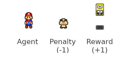
In this post we will consider a simple discrete and turn based 2D environment, in which a single agent (let’s take Mario to make the whole thing more visually appealing) can perform one of these four actions each turn: going right, left, up or down. Mario will receive a reward each time he finds a block, and a penalty each time he encounters a goomba.

Q-value and policy

Now let’s put ourselves in the shoes of Mario, imagine an even simpler 1D environment where there is a block two steps away on the right side while there is nothing on the left.

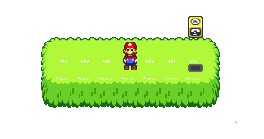
The optimal policy is pretty straightforward: always go right. But how do we know it for sure?

Well, nether going right or going left will earn Mario any reward, however we have the intuition that he should be going right because he will then be only one step away from the block. In other words, the position one step away in the right direction is of higher “quality” than the one one step away in the left direction. We call these quality values the Q-values.

Estimating the Q-values of each action for a given state of the environment is at the core of a whole class of RL algorithm, we are going to study a few of those.

We can compute the Q-value of a given action a in a given state s with the Bellman equation:

Where Q(s, a) is the Q-value of action a in state s, R is the reward Mario gets by taking such action and s’ is the state he ends up in. The term π(s’, a’) is the probability of choosing action a’ when the agent is in state s’. π stands for policy, it is the function that determines the behavior of the agent.

The meaning of this equation is exactly what we talked about earlier: the quality of a given (state, action) pair is equal to the reward Mario gets by executing that action in that state, plus the quality of the next (state, action) pair available (weighted by the policy).

You may also have noticed the γ factor that weight the quality of future Q-Values in the above formula, it is called the discount factor and is a quantity between 0 and 1, but more on that a little later.

In fact, our toy example is simple enough so that we can solve the Bellman equation by hand, no need for a complex algorithm. Let’s do it: grab a piece of paper!

Pen & Paper 1: Solving the Bellman Equation

Just kidding, it will be quick and painless: I will do it for you ;)

First we need to decide on a policy, the easiest one is to always pick the best possible action: it is called the greedy policy. Let’s put it in our Bellman equation, we just need to replace the sum by a max (because in this case π(s’,a’) = 1 if the choice is optimal, 0 otherwise).

We can start by the end: when Mario reaches a block the game is over, so basically for each action leading to a block Q(s, a) = R = 1.

Now for an action that leads to an empty state (no goomba or block), the reward is zero, then Q(s, a) = γ max(Q(s’, a’)).

So if an action a lead us to a state one step away of a block, the next best action is to reach the block and it has a Q-Value of 1 as we computed just earlier, and Q(s, a) = γ * 1 = γ

Similarly, if we are two steps away from a block, walking toward the block earn us a reward of 0, but the next best action has a Q-Value of γ, thus if we are two steps away and walk toward a block: Q(s, a) = γ².

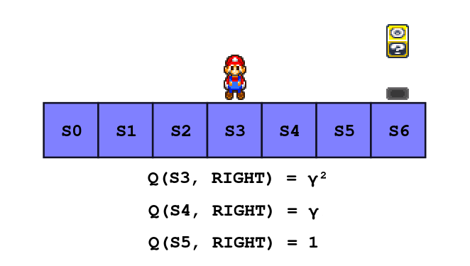
Can you guess what would be the Q-Values Q(S5, LEFT)? Yes γ² exactly, because if Mario is in state S5 and goes left he will end up in S4 where we already know that the best action is to go right with a Q-Value of γ.

Sarsa

Now we suppose that the agent has no prior knowledge of the environment, thus the agent can’t compute the exact Q-values as we did before. What we are going to do instead is to estimate the Q-values by updating them accordingly to our observations while exploring the environment.

We will use the Sarsa algorithm to learn Q-values and improve the behavior of the agent over time. Sarsa is a reinforcement learning algorithm that lay the foundations of a whole class of more evolved reinforcement learning algorithms. Having a deep understanding of Sarsa will actually help you to grasp advanced RL concepts more easily.

The algorithm is the following:

Q = zeroed_q_values
γ = discount_factor
η = learning_rate
next_s = initial_state
next_a = choose_action(Q, initial_state)

while (True):
	s = next_s
	a = next_a
	r, next_s = take_action(s, a)
	next_a = choose_action(Q, next_s)
	
	Q[s][a] += η*(r + γ*Q[next_s][next_a] - Q[s][a])

In plain words: we start at state s, take an action a, observe a reward r and the next state s’, we take another action a’ and then we can update the Q-Values by the quantity ΔQ(a, s) computed by:

This update rule gives us the guaranty that if all Q-values have converged in expectation (that is ⟨ΔQ(a, s)⟩ = 0), then our Q-Values are solutions of the Bellman equation.

If you are wondering why this algorithm is named Sarsa, the answer is the following:

The name sums up all the steps of the algorithm, well almost, don’t forget the update at the end… Maybe we should call it Sarsau 🤔

But enough theory, I promised you an interactive introduction to reinforcement learning, the time to fulfill my promises:

(If the iframe is not loading for some reason, try to refresh the page or check it here)

You can start the simulation by clicking the leftmost button, you will see the agent (Mario) walking randomly. Mario is following a greedy policy in this first example, but because at the beginning all Q-Values are 0, he chooses actions randomly.

The color map depict the Q-Values, it will be updated for the first time when Mario finds either a block or a goomba (because before that all received rewards are zero, as well as all Q-Values, check the update rule).

In this case the Q-Values are stored in a 3d array indexed by x and y positions, as well as actions: Q(x, y, a). To keep visualization simple, each square of the color map is divided into 4 triangles, representing the 4 actions possible in each state. Thus, the leftmost triangle of the square (x, y) represent Q(x, y, LEFT), the topmost Q(x, y, UP) and so on.

A fuchsia triangle indicates an action with a high Q-value, while cyan stands for low (negative) Q-values.

To see those Q-values appear you can speed up the agent (middle button) instead of waiting. You can also reset Q-values to observe the agent re-learn for scratch, this will be especially useful in the upcoming environments because of the probabilistic nature of reinforcement learning, always run a few simulations before making any conclusion.

Exploration vs Exploitation dilemma

You may have noticed that the agent will quickly find a path that leads to a reward, however if you are unlucky that path may not be optimal, in that case the agent will stubbornly execute the same sequences of suboptimal choices over and over again. The agent is not aware of the existence of a better path, it just exploits its current knowledge of the environment.

To improve its behavior, the agent should sometime explore and look for better options. Choosing between both option is what we call the exploration vs exploitation dilemma.

The greedy policy leave no room for exploration: the best action - based on the current knowledge - is always selected.

Fortunately, there are other policies that encourage more or less exploration. One of these is called ε-greedy: with a probability ε the agent takes a random action, otherwise it fallbacks to the usual greedy policy.

The softmax policy is another well known example: it weights each action accordingly to its estimated Q-Value:

Note that the softmax policy introduce a parameter, β, whose impact depends on the actual value of the Q-Values, itself depending on the rewards and their distributions in the environment. In other words, if you decide to double both rewards and penalty this will impact the behavior of an agent following a softmax policy, but there will be no change for an agent using ε-greedy.

It’s better if you judge by yourself: this time I’ve put a red block that is only worth 0.5 points while the yellow one is still worth 1 point. It’s easier to get the first, but if the agent explores a little more it may find out that it’s not the best option. Don’t be shy to try huge epsilon or small beta to force random exploration, once you are done exploring switch to greedy policy by setting epsilon to 0.

A few words on parameters

In fact, what I just said about a block further away but giving twice the reward being a better option is not always true, it depends on γ, the discount factor.

Remember when we solved the Bellman equation earlier? We found out that if an action put the agent in a state one step away from a block (with a reward of 1 point) it’s Q-Value is Q(s, a) = γ, if it’s two steps away Q(s, a) = γ², and extrapolating, if it is n steps away Q(s, a) = γⁿ.

The general formula in our particular set up, with the greedy policy and with a reward r is Q(s, a) = γⁿ * r. This mean that if you set the discount factor to 0.5, a reward of 2 has the same perceived value than a reward of 1 one step closer to the agent.

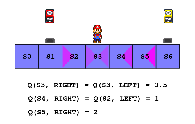
The lower the discount factor, the more the agent will go for short term rewards. Conversely, a discount factor close to 1 will much less penalize the agent for long term planing, or for taking a few days off. It’s your job to pick the right value for your use case.

Another parameter I didn’t talk about is η, the learning rate. If you already have a machine learning background you might be used to it, otherwise it is exactly what you think it is: the rate at which the agent is learning.

Set it too high and the Q-values will oscillate (even if a good path is found it can be unlearned very quickly), set it too low and the agent will take ages before learning anything. A common strategy is to start with a rather high value and progressively bring it down to a final, rather low learning rate.

As always, when it comes to picking parameters it is up to you to strike the right balance.

To let you play with the discount factor the red block (worth 0.5 points) is still there. Pick a value for γ and check which block the agent choose (don’t forget to explore!). You can also try extreme values of learning rate and see what happens. Just be curious!

Multi-steps Sarsa

If you read that far I guess that you spend some time watching the agent evolve in its environment, you may have been annoyed by the fact that the agent needs to complete a few episodes before learning a complete path. In fact if a reward is n steps away, the agent needs at least n episodes before information about the reward reach the initial state.

We can do better, for instance we can change the update rule to actually update the Q-value after two steps instead of one:

The algorithm with the updated rule is called 2-steps-Sarsa. Now the agent needs to take two steps before being able to update the Q-Value: start in s, take action a, observe reward r and get to s’ then again take action a’, observe reward r’ and get to s’’, finally take action a’’ and update.

Yep, you can call it Sarsarsa if you want to.

In the end, what this new update rule means is that when the agent updates its Q-Value Q(s, a), it will take into account the two next rewards and the Q-Value two steps further, Q(s’’, a’’), that is the quality of the situation two steps away from s.

Intuitively, the agent will propagate the information two steps back each time. Thus, if a reward is 4 steps away, the agent needs only 2 trials to propagate information back to the initial state (assuming that it follows two times the same path).

Obviously Sarsa can be generalized to take any number of steps into account, the update rule for n-steps-Sarsa is:

From a practical view, to implement n-steps-Sarsa you need to keep track of the n last states, actions and rewards, but other than that the algorithm is very similar.

If all of this is still a little confusing, it will hopefully become much clearer with an example:

Q-Learning

I know that there is already a lot to digest, but would like to talk about one last variant of Sarsa: Q-learning.

Remember the Bellman equation? I paste it here again so that you don’t need to scroll up:

Here π is the policy. Ideally in the end we want to pick the greedy policy, however as we discussed before we need to pick a policy that allows the agent to explore, for instance ε-greedy.

It is important to understand that the policy we choose decides the “real” Q-values that we are trying to estimate with Sarsa. Thus, if the agent is trained with a policy that is not the greedy policy it will learn a suboptimal behavior, because that behavior takes into account the fact that the agent can make mistakes.

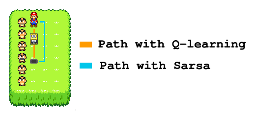
An example is worth a thousand words, imagine that our agent is walking alongside a cliff and receive a negative reward if it falls. In our setting let’s say that Mario is walking alongside a line of goomba instead:

The reward is right there on the cliff edge. With the greedy policy there is no risk of falling because the agent always pick the best action, thus Q-values along the cliff will be high.

However, if the agent follows an ε-greedy policy there is a risk of falling when walking on the edge, thus Q-Values along the cliff will be lower in that case. If the agent can make mistakes, staying one step away from the edge is much safer and that path is only 2 steps longer, Q-values might be higher there.

So what if you want to learn the optimal path? You can’t really use the greedy policy with Sarsa because without exploration there is too much of a risk of staying stuck with a suboptimal path. That is where Q-Learning comes in.

The Sarsa algorithm is what we call an on-policy algorithm, because it learns with the same policy that dictates its behavior. Whereas Q-Learning is an off-policy algorithm, it uses the greedy policy to learn but its behavior follows another policy during training, for instance ε-greedy.

In other words, Q-learning allows the agent to learn the Q-values corresponding to the greedy policy (the best one) while still allowing it to explore by following a probabilistic policy during training.

More formally, Q-learning estimates the Q-Values for the Bellman equation with the greedy policy:

But actually follows a policy that allows exploration. Thus, it uses a slightly different update rule than Sarsa:

As you can see, the only difference is that we do not update the Q-Value using the next chosen action a’ (based on the current non-greedy policy) but with the best possible action a*, as if we used Sarsa with the greedy policy.

Let’s just see how it works in practice: try to use Q-learning with ε-greedy and when the agent has learned for long enough switch to the greedy policy (set ε to 0). What is the difference with Sarsa? You can try different values of ε.

One big question remains: when to use Sarsa over Q-Learning or Q-Learning over Sarsa?

With Q-Learning the agent takes more risks, but learns an overall better policy. If you are creating an IA to beat a game with the higher possible score, go for Q-Learning and switch for greedy policy once the agent is trained.

Sarsa is a safer approach, it learns optimal Q-Values knowing that the agent can make mistakes. With Sarsa the agent will take much fewer risks during training, it is a good choice for online training in customer facing application for instance. Sarsa is also more suited for always-learning algorithms, because you can stick with a policy that allows exploration and still have good performances (which is not what is optimized with Q-Learning!).

Real world applications

Maybe you are starting to get a bit bored watching Mario searching for blocks, but don’t worry I have got your back: now is the time to discuss other, more practical applications.

We will study two use cases: playing Super Marios Bros (oops Mario again, sorry I couldn’t resist the temptation) and deciding of the best moment to prompt a user to take an action, say buy a coffee.

My goal in this section is to give you a feel of what is actually feasible, what is not and how to tackle a given tasks in the light of what we discussed in this post. Sadly it seems to me that this part is missing in a lot of posts on reinforcement learning, I hope you will find it useful and that it will inspire you to put some RL in your own applications!

Super Mario Bros

Let’s start with the hardest task first: we want to train an agent to play Super Mario Bros, the agent should be able to complete as many levels as possible.

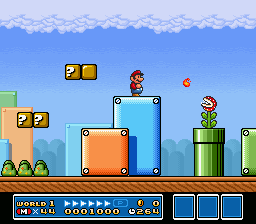
To apply Sarsa or Q-Learning we first have to decide on two things: what are the actions and what are the states?

Regarding actions, the game uses 3 directions (UP does nothing) and 2 buttons A and B. At given time you can press either zero or one direction, and either no action button, only A, only B or A and B. That is a total of 16 distinct actions to choose from.

Note that it is better to keep this number as low as possible: there is in total 64 (6 buttons thus 2⁶) possible actions, but most of them are redundant and thus would increase by a factor of 4 the number of Q-Values our agent needs to learn for nothing in return. This is due to the fact that Sarsa can not generalize what it learns from a given action to others by itself.

Now what about the states? The first level alone is roughly 100 blocks long for 20 blocks high, if we encode the state with the agent position (x, y) that is about 2.000 states, but enemies are moving too! Plus this doesn’t generalize to other levels.

Let’s try something else, we can discretize the surroundings of Mario and encode only that part of the world:

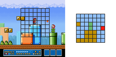
Let’s say we take a 7*7 square centered around Mario, each block can be either empty, solid (a brick or the ground), an enemy Mario can’t jump on (a fire ball, piranha plants), an enemy Mario can jump on (a goomba, a koopa) or Mario itself. Yes you guessed it right, that is already are 5⁴⁹ distinct states with an overly simplified solution. Spoiler alert: it does not fit into memory.

That is the actual limit of Sarsa and Q-Learning: the number of state grows really quickly, often too much to be practical. That is where neural network based algorithms such as Deep Q-Learning & Co shine, but that is a story for another time.

Let’s not surrender that easily, I expect the actual distribution of states to be very sparse: that is some of them will appear very often while others will probably never show up. In fact after googling a little while I found a report from a student project that used a similar approach and reported about 20000 states in their final table. That is still a lot but at least if we store only states Mario actually encounters it should be tractable on any modern personal computer.

Ok suppose that we can deal with that many states, should we use Q-learning or Sarsa? We only care about the final score, we are looking for the best possible policy and don’t mind the agent’s death during training, thus we should be going for Q-learning.

What about rewards? I see two approach here:

• We can compute the closest distance from the end of the level achieved for the current run and give the agent a reward each time he improves that distance.
• We can give the agent a reward when it completes the level. However, the agent is very unlikely to complete the level randomly in the first place, to compensate a good idea is to have the agent start at a random location in the level, this will help it to explore much faster and hopefully it will be able to complete the level a first time when starting close enough of the end.

In both case we can give the agent a penalty each time it died.

Would you like to add a cup of coffee?

Now let’s try to do something much more realistic and practical: imagine you run an online store, a blog or a restaurant where customer make orders on a terminal, you probably want don’t want your customers/visitors to miss a T-shirt they could like, your future post or the button hidden at the bottom to order a coffee, what about using a prompt?

However, you are probably annoyed by all those prompts everywhere as much as I am. If you don’t want to bother your customers too much you can try to predict when the prompt will actually be useful for them and are likely to take the action.

How can we frame this task as a reinforcement learning problem and train an agent to decide when to fire the prompt?

First the actions, there are two of them: fire the prompt or do nothing, easy.

Then the states, let’s study two cases, a blog and a restaurant:

• For you blog you want your visitor to subscribe to your newsletter, what types of visitor usually subscribes? Probably those that spend some time reading your articles, visit many pages and come back. The tuple (reading time, page viewed, number of visits) is probably a good indicator. However, to keep the number of state low it is better to discretize, for instance you can encode reading time by one of:
  • Less than 5 minutes
  • Between 5 and 10 minutes
  • between 10 and 30 minutes
  • between 30 minutes and 1 hour
  • more than 1 hour
• Now you are running a restaurant that boast a choice of 10 starters, 10 main courses and 10 deserts, and you want to propose a coffee while the customer is composing its order. That is a total of 1000 states, if your restaurant is big enough you can cope with that, otherwise consider grouping some meal together.

You give a reward to the agent each time he prompt the user and get a positive response, otherwise if the response is negative you give it a penalty.

In this use case you are dealing with real customers, you can’t afford the agent to do whatever it wants while learning. In such scenarios it is better to use Sarsa over Q-learning, remember the cliff? Sarsa will play safer.

If you already have data about your customers it is even better: you can pre-train your agent before putting it in front of real people. It may also be reasonable to put hard-coded safeguards, to avoid the agent spamming users for instance.

Hope it gives you some ideas!

Conclusion

And that’s it, I know that this a long post, but I really wanted to cover all that material, from a little of theory to practical use cases, to give you a good first picture of reinforcement learning.

Obviously the field of reinforcement learning is much bigger than what I depicted here, we don’t even talked about neural networks even though they are powering all current state-of-the-art algorithms such AlphaGo to quote just one.

Anyway I hope you found it interesting, that you’ll give a try to RL, and that you will be able to build up on what I shared here.

If you find any mistake don’t hesitate to report it here, otherwise I hope to see you next time!